
Propensity models are a common type of predictive model in machine learning, especially in marketing, customer analytics, sales, and healthcare. They estimate the probability (propensity score) that a person or entity will take a specific action in the future, based on historical data and patterns.
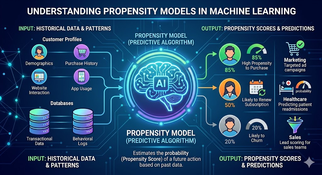
What is a Propensity Model?
A propensity model predicts the likelihood of a binary outcome (yes/no event), such as:
- Propensity to buy / convert / purchase a product
- Propensity to churn (cancel subscription)
- Propensity to click, engage, upgrade, renew, or respond to an offer
- Propensity to default on a loan (in finance)
The output is usually a score between 0 and 1 (or 0%–100%), representing the predicted probability for each individual.
From a machine learning perspective, this is typically framed as a binary classification problem (though the focus is more on well-calibrated probabilities than hard 0/1 decisions). Common algorithms include:
- Logistic Regression (simple, interpretable baseline)
- Random Forests, XGBoost, LightGBM (powerful tree-based ensembles)
- Neural networks (for complex data)
- Sometimes Bayesian methods or stacking ensembles
Key distinction: In causal inference, “propensity score” often refers specifically to the probability of receiving a treatment (e.g., in observational studies to reduce confounding). In business/ML contexts, it more broadly means any probability of a future customer behavior.
How Propensity Models Are Built
- Define the target — e.g., “Did the customer purchase within the next 30/60/90 days?”
- Feature engineering — Use behavioral data (page views, past purchases, RFM metrics, demographics, engagement signals, etc.).
- Train the model — On historical data where the outcome is known.
- Score new records — Generate propensity scores for current customers/leads.
- Deploy & monitor — Scores feed into segmentation, targeting, personalization, or prioritization.
Important Evaluation Metrics for Propensity Models
Standard classification metrics apply, but business-oriented ones like lift/gain are especially critical because the goal is usually targeting efficiency (identifying high-propensity customers to maximize ROI).
1. Discrimination / Ranking Metrics
- AUC-ROC (Area Under the Receiver Operating Characteristic Curve): Measures how well the model ranks positive cases higher than negative ones.
- 0.5 = random
- 0.7–0.8 = decent
- 0.85–0.9 = strong (depending on domain)
- Very popular for propensity models.
- Precision-Recall AUC (PR-AUC): Better when the positive class is rare (e.g., purchase rate is only 2–5%).
2. Calibration Metrics
Propensity models need well-calibrated probabilities (a score of 0.8 should mean ~80% actual chance).
- Brier Score — Mean squared difference between predicted probability and actual outcome (lower is better).
- Reliability diagrams / Expected Calibration Error (ECE).
3. Business-Oriented Metrics (Most Important for Marketing/Sales)
- Lift / Uplift Charts:
- Sort customers by predicted propensity (highest to lowest).
- Divide into deciles/ventiles (e.g., top 10%, top 20%).
- Lift = (Response rate in top X% ) / (Overall response rate).
- Example: If top 5% has 7x higher purchase rate than average, lift = 7.
- Cumulative Gains Chart: Shows what % of total positive outcomes you capture by targeting the top X% of scored customers.
- KS Statistic (Kolmogorov-Smirnov): Maximum separation between cumulative distributions of positives and negatives.
4. Other Useful Metrics
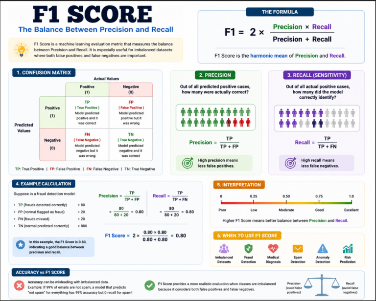
- Precision, Recall, F1 at specific operating thresholds (e.g., you might target only scores > 0.7).
- Log Loss (Cross-Entropy) — Good for probabilistic calibration.
Note on Propensity vs. Uplift Models: Pure propensity predicts “who is likely to buy.” Uplift models (or incremental response models) predict “who is likely to buy because of our intervention.” Uplift uses different evaluation (Qini coefficient, uplift curves).
Practical Tips
- Class imbalance is very common — use techniques like SMOTE, class weights, or focal loss.
- Backtesting / Time-based validation is crucial (avoid leakage from future data).
- Interpretability matters — use SHAP/LIME values to explain why someone has high propensity.
- Monitor drift — Customer behavior changes, so retrain periodically.
- Start simple (logistic regression) for baseline and explainability, then move to gradient boosting for performance.